
How to Implement Factorized Attention for Time Series
Self-attention time-wise and space-wise for time series data

Yesterday I explained the concept of factorized attention – splitting normal attention into time-wise and space-wise components.
Today, let's actually implement this in PyTorch.
If you prefer video:
The process of self-attention
To do this, we take our raw time series and turn it into a numerical representation that captures it's own meaning and includes relevant context.
The process looks like this:
Embedding representation: Convert the time series patches into vectors
Linear transformations: Create Query, Key, and Value vectors for each token using the Query, Key, Value matrices that are learned by our model
Vector dot products: Measure similarity between tokens
Softmax normalization: Convert similarities into probability weights
Context vector: Use the weights and Value vectors to get the updated vectors now with contextual meaning mixed in
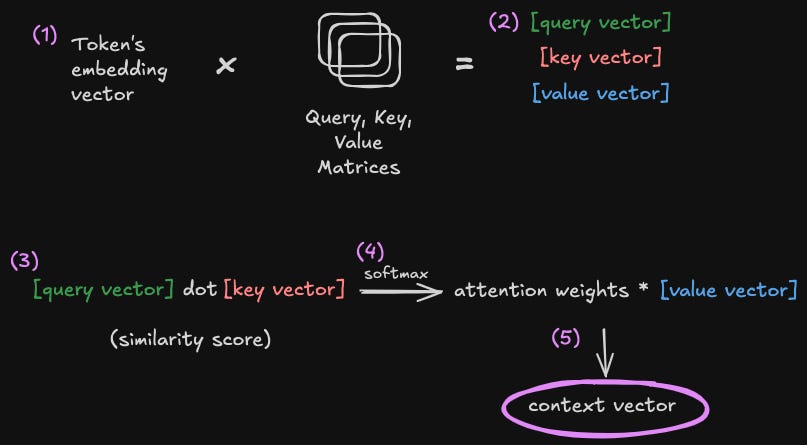
The context vector is the output of our Transformer block.
It is then either passed to another Transformer block where the same process repeats or finally passed to our feed-forward layers of the model to predict an output.
Factorized self-attention
In factorized attention, we keep the structure and process:
First time-wise: attention within each stock's time sequence
Then space-wise: attention across stocks at the same time position
The only difference between “regular” self-attention and time-wise self-attention here is the shape of the input tensor. If we wanted to do “regular” attention we would flatten our data into a single time series of 40 patches x 128 dimensions each instead of 4 different channels with 10 patches.
The key distinction between factorized self-attention and regular attention is this preserving of structure between space and time.
The tensor shape conceptually
A tensor is a nested array of arrays for organizing our data to train.
For Transformers the tensor shape conceptually looks like this:
batch size: number of independent examples
channels/variates: the different features (stocks)
sequence of tokens: the ordered elements to attend over
dimensions of tokens: the embedding size for each token
The basic tensor shape:
(batch size x channels x tokens x dimensions)
For our examples we will use a batch size of 1 to make things simpler.
The embedding tensor for time-wise and space-wise attention
This part took me awhile to wrap my head around.
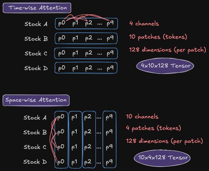
The time-wise input tensor for our example is:
(4 stocks x 10 patches x 128 dimensions)
4x10x128
Each stock is it’s own independent time series (channel). We have 10 tokens (patches of timesteps) in each channel. And each token is 128 dimensions in the embedding space (128 values in an array to capture the meaning of the token).
The space-wise input tensor would be:
(10 channels x 4 patches x 128 dimensions)
Here each patch time is it’s own independent channel. We have 10 different time steps we want to compare how the patch for each stock across this time step impact each other. So we have 10 channels.
Each channel is the patch/token from each of our 4 stocks and this sequence is what we compute attention for. Again each patch having 128 dimensions.
Step-by-step time-wise attention calculation
Let's walk through how attention actually works, using our example from yesterday with 4 stocks and their price movements. For convenience the data is randomly generated.
This initial example is doing time-wise self-attention where each stocks time series is treated independently.
Our input embedding is combining 10 patches from 4 different stocks into a single tensor.
A patch being our token which is just a slice of N timesteps from the raw data.
1. Initial Embedding
Each patch of time series data gets converted into a vector:
# For 4 stocks with 10 time patches each into a 128 embedding dimensional space

embeddings = torch.randn(4, 10, 128)  # Shape: [4, 10, 128]
2. Query, Key, Value Projections
Our Transformer model is initialized with a Query, Key, and Value matrix in each attention head. These matrices are updated throughout the model training process.
The size of these matrices are determined by the model architecture.
We transform each embedding into three different vectors using learned weight matrices:
# Create projection matrices
W_query = torch.randn(128, 64)  # embedding_dim -> query_dim
W_key = torch.randn(128, 64)    # embedding_dim -> key_dim
W_value = torch.randn(128, 128)  # embedding_dim -> value_dim

# Project embeddings to Q, K, V
Q = torch.matmul(embeddings, W_query)  # Shape: [4, 10, 64]
K = torch.matmul(embeddings, W_key)    # Shape: [4, 10, 64]
V = torch.matmul(embeddings, W_value)  # Shape: [4, 10, 128]
3. Attention Scores and Weights
Now we compute how similar a query for a token (what am i looking for) is with the key of every other token (what info I offer).
This gives us a set of weights that shows how much a token cares about another token.
# Transpose K for matrix multiplication
K_transposed = K.transpose(-2, -1)  # Shape: [4, 64, 10]

# Compute attention scores
# Q @ K_T shape: [4, 10, 10]
attention_scores = torch.matmul(Q, K_transposed)

# Scale scores by square root of key dimension
attention_scores = attention_scores / (64 ** 0.5)

# Apply softmax to get weights that sum to 1
attention_weights = torch.softmax(attention_scores, dim=-1)  # Shape: [4, 10, 10]
4. Context Vector Creation
Finally, we use these weights to create a weighted sum of values:
# Weighted sum creates the context vectors
# Shape: [4, 10, 128]
context_vectors = torch.matmul(attention_weights, V)
Space-wise attention calculation
The process is the same as above, we just reshape the context vectors with the time data into our space-wise input embedding.
1. Initial Embedding
Reshaped the output of our time-wise context vectors. Remember, we now want each of the 10 time patches to be separate channels with a sequence length of 4 patches (for each stock).
This will enable us to compute attention across each stock.
space_embeddings = time_context.transpose(0, 1) # shape: [10, 4, 128]2. Query, Key, Value Projections
We define new weight matrices for space-wise attention (they can be different from the time-wise). Then project our space embeddings as well.
W_space_query = torch.randn(128, 64)
W_space_key   = torch.randn(128, 64)
W_space_value = torch.randn(128, 128)

# space_embeddings.shape = [10, 4, 128]
space_Q = torch.matmul(space_embeddings, W_space_query)
space_K = torch.matmul(space_embeddings, W_space_key)
space_V = torch.matmul(space_embeddings, W_space_value)
3. Attention Scores and Weights
Now we compute how similar a query for a token (what am i looking for) is with the key of every other token (what info I offer).
This gives us a set of weights that shows how much a token cares about another token.
# space_Q: [10, 4, 64]
# space_K.transpose(-2, -1): [10, 64, 4]
# => space_scores: [10, 4, 4]
space_scores = torch.matmul(space_Q, space_K.transpose(-2, -1)) / (64.0 ** 0.5)
space_weights = torch.softmax(space_scores, dim=-1)  # shape: [10, 4, 4]

# Weighted sum over values => [10, 4, 128]
space_context = torch.matmul(space_weights, space_V)
4. Context Vector Creation
Finally, we use these weights to create a weighted sum of values:
# Weighted sum over values => [10, 4, 128]
space_context = torch.matmul(space_weights, space_V)
5. Transpose back
# shape: [10, 4, 128] -> [4, 10, 128]
space_context = space_context.transpose(0, 1)
print(space_context.shape)
Next Steps
Depending on the model architecture this attention calculation can be repeated multiple times. The code above is simplified for illustrative purposes. In practice there are multiple layers with feed-forward blocks, skip connections, normalization, and many more attention heads.
Eventually the context vectors, now imbued with all the meaning from the various attention calculations, get’s passed to a neural network of some kind to output a prediction.
During training this prediction is then measured against some expected output, the loss is calculated, and then the gradients are computed for each parameter. This gradient shows the direction to “nudge” each parameter that would reduce the loss.
This cycle happens many times until the model is trained.
That’s a deep dive for a different day.
View all related code here on my GitHub.